Computational Fabrication Final Project: Terrain from Audio

Introduction

This project aims to use audio as an input to generate 3D terrain. Audio signals can be decomposed into their constituent frequencies using Discrete Fourier Transforms (DFTs). Performing DFTs over consecutive windows in the audio signal gives a series of lists that contain the frequency amplitude outputs. Taken altogether, this gives 3 dimensions of data to be used for generating terrain:

1. Time
2. Frequency
3. Amplitude

Time and frequency will be used to index a specific point in 2D grid space, and the amplitude will generate the actual terrain in the z-dimension. This can be thought of as displacing the vertices of a mesh up or down. Then, considering the large range of possible amplitudes, the resulting landscape will be interpolated to a reasonable range and smoothed using a Gaussian filter.

In addition to generating terrain from a plane, a sphere mesh will be used as well. I wanted to try this for generating planet-shaped objects. This was inspired by one of my favorite games, Outer Wilds, which features a miniaturized solar system comprised of planets with exaggerated terrain features.

For displacing the vertices of a sphere mesh, polar coordinates must be used. The amplitude will correspond to the radius instead of the z-dimension.

I used Rhino and Grasshopper for this project. I also wrote a Python script component in Grasshopper that reads and processes the audio data.

Materials

Generic PLA material was used in the printing process. The materials and Prusa Mini printer were provided by the BTU Lab of the University of Colorado Boulder.

Reading and Processing Audio Files with Python

In order to read audio, the data must be in a WAV file first. The Python script I wrote uses the SciPy library to read the audio, process it with a Fast Fourier Transform (FFT), and pass a Gaussian filter over the displacement matrix. NumPy is used for any intermediate array operations. The script is shown below. It takes a variety of inputs supplied by the Grasshopper script to allow for quick parametric design of the output.

The outputs of the above script are two lists whose lengths match the number of vertices in the according mesh. In the planar case, a single vertex is transformed up or down by its corresponding value in the list. Because the list was originally a matrix with the rows representing the time step, this results in a surface physically representing the shift in frequencies over time.

Generating Terrain with Data in Grasshopper

Within Grasshopper, a fair amount of work needed to be done to transform a list of values into actual 3D-printable objects. My script is divided into 5 sections:

1. Python script for processing the audio and its input parameters
2. Creation of displaced planar mesh
3. Addition of solid base to planar mesh
4. Creation of displaced spherical mesh
5. Transformation and joining of both objects for baking into Rhino

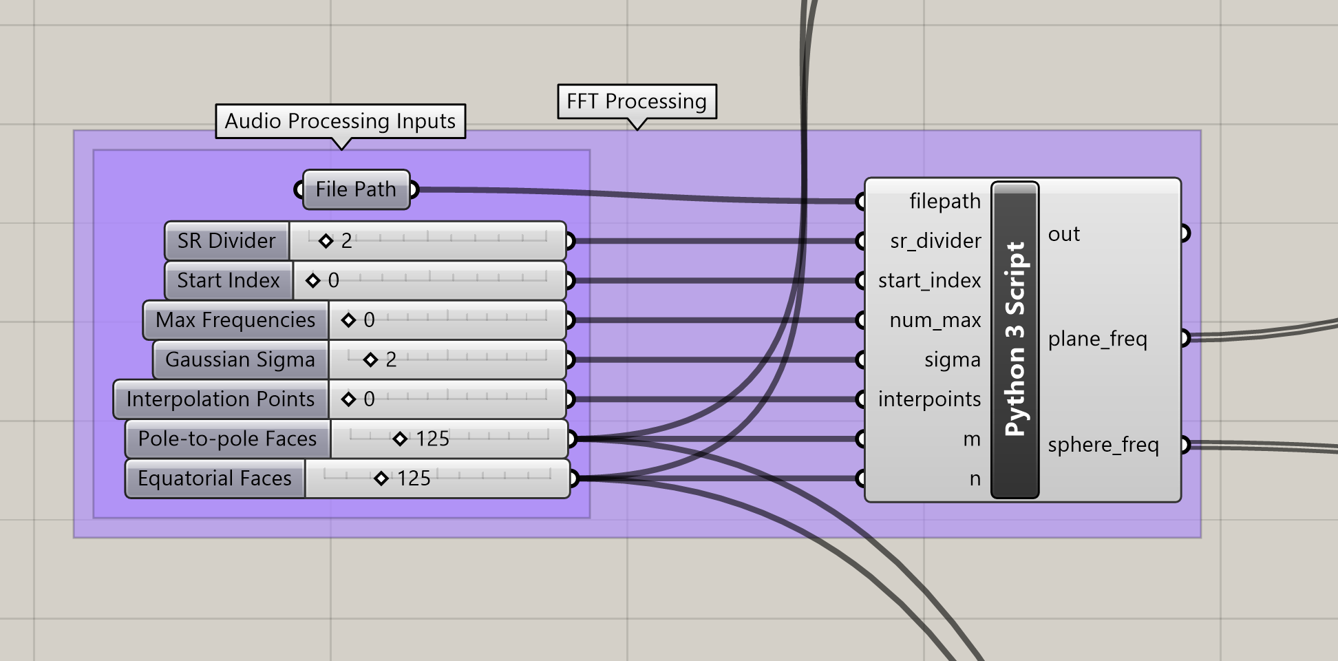
Starting off, let us look at the Python script component in Grasshopper. Outside the code itself, the component is simple and offers a compact location to edit the starting parameters.

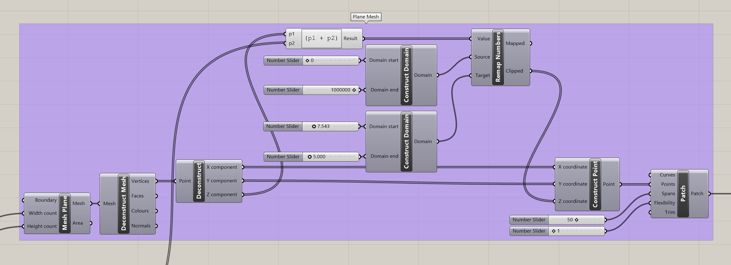
In the Plane Mesh group, the length (m) and width (n) values are used to construct a mesh plane that is subsequently deconstructed into its vertices. The processed Python outputs are added to the z-values of the vertices and interpolated to a parameterized range. Finally, the resulting points are patched together into a single mesh again.

Next, the Base Creation group performs some tedious boolean operations to create solid base for the terrain to rest on.

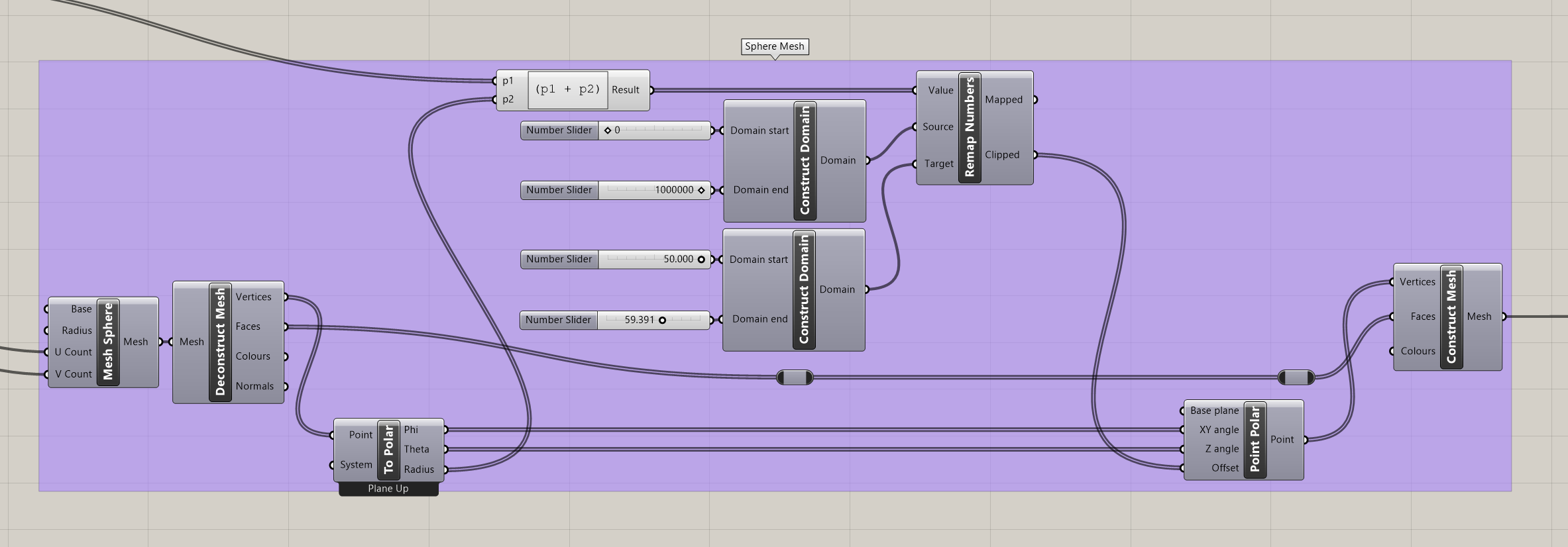
On the other side, the Sphere Mesh group starts from a sphere mesh and displaces the vertices radially using polar coordinates from the deconstructed mesh. Just like with the planar case, these values are mapped to a reasonable range to prevent sharp points that would be troublesome to print.

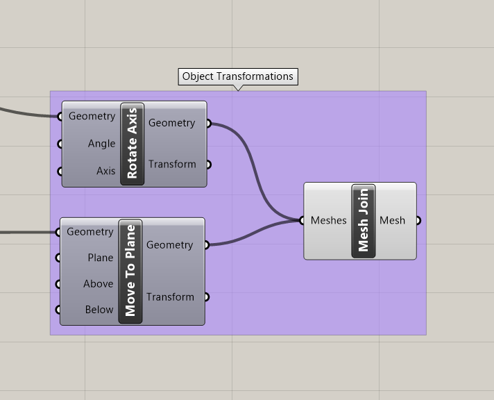
Finally, both objects are transformed to lie on the XY plane and joined in one component. Following this, right-clicking the component while a suitable parameterized design has been selected will bring up an option to bake the output. Baking the two objects will render the objects directly in Rhino and allow them to be selected as such. With both selected, they can be exported as an STL file, which is sent to the slicer for generating G-code to be used in 3D printing.

Here’s the Grasshopper script in its entirety. I left the parameters at the values that most often produced good results. Download the full Grasshopper file here.

Outputs

Below are a few examples of various outputs rendered in Rhino.

Generated with Vital Tides by Thomas Happ.

Generated with Travelers by Andrew Prahlow.

Generated with Heart by Plini.

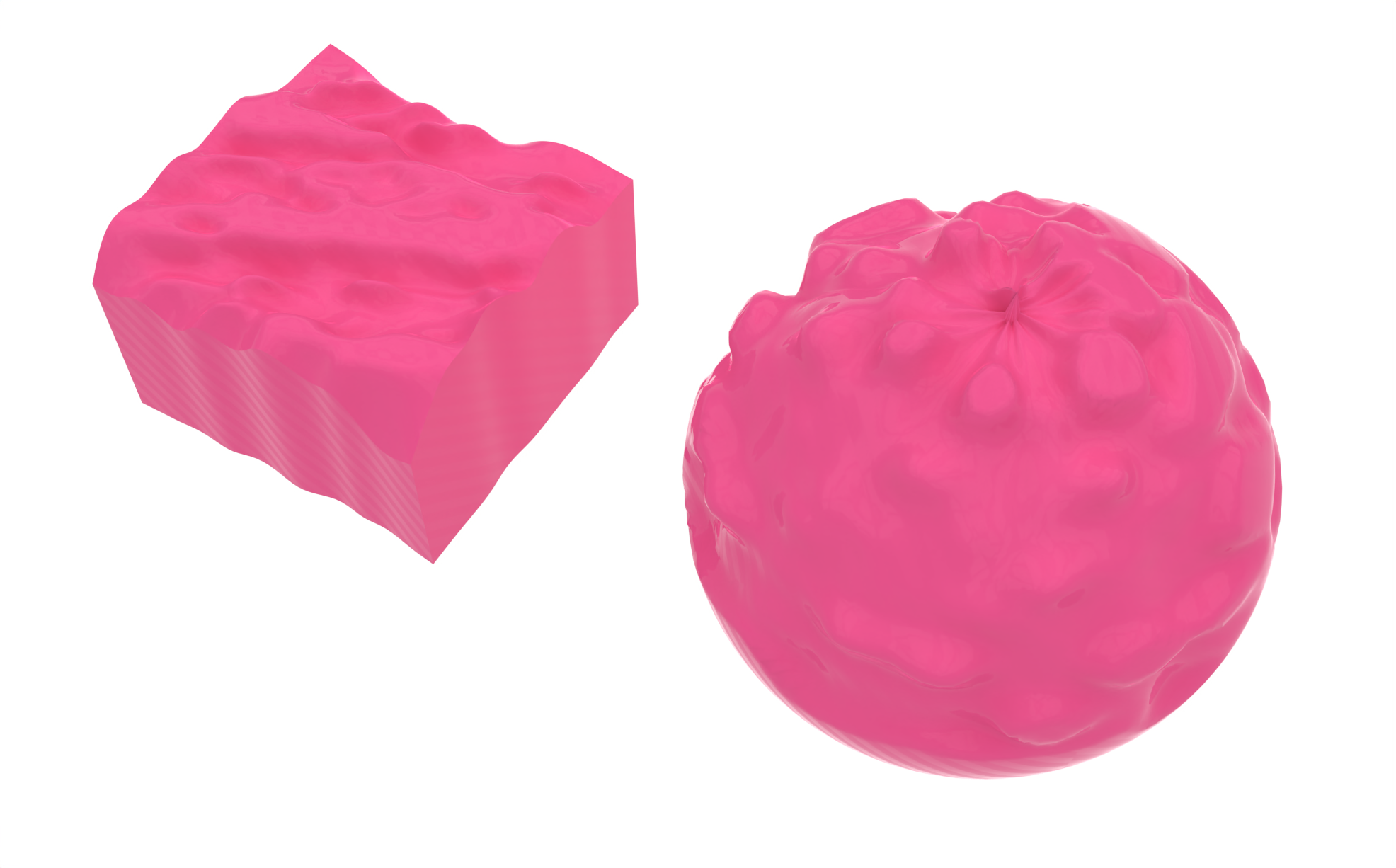
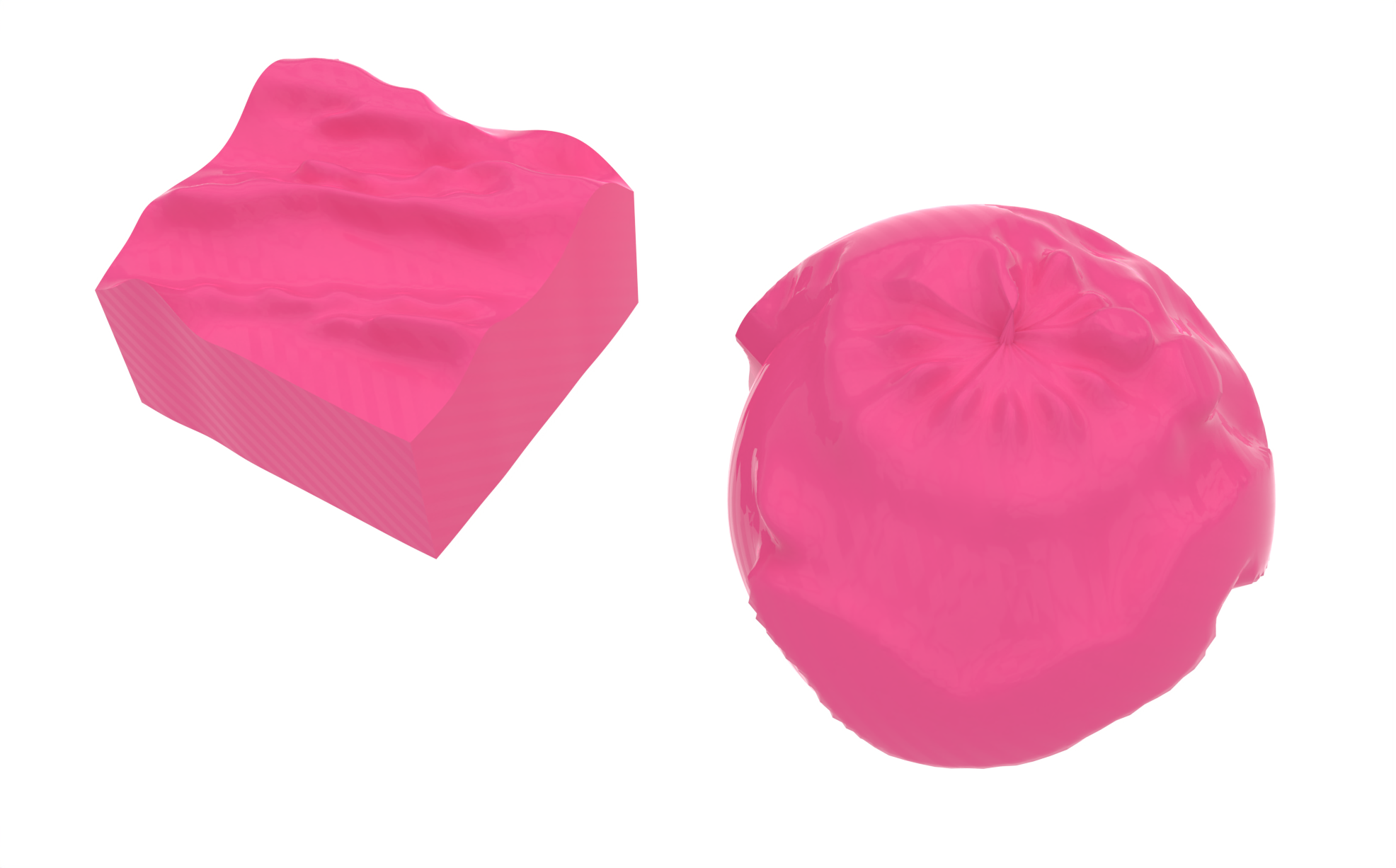
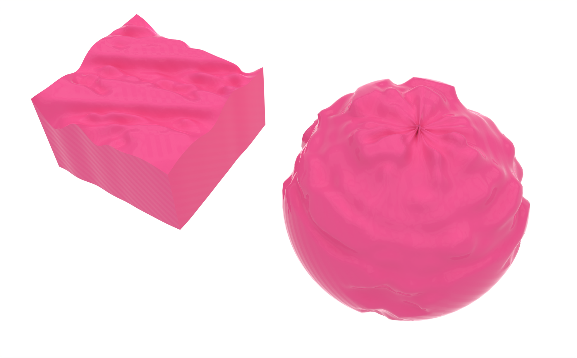
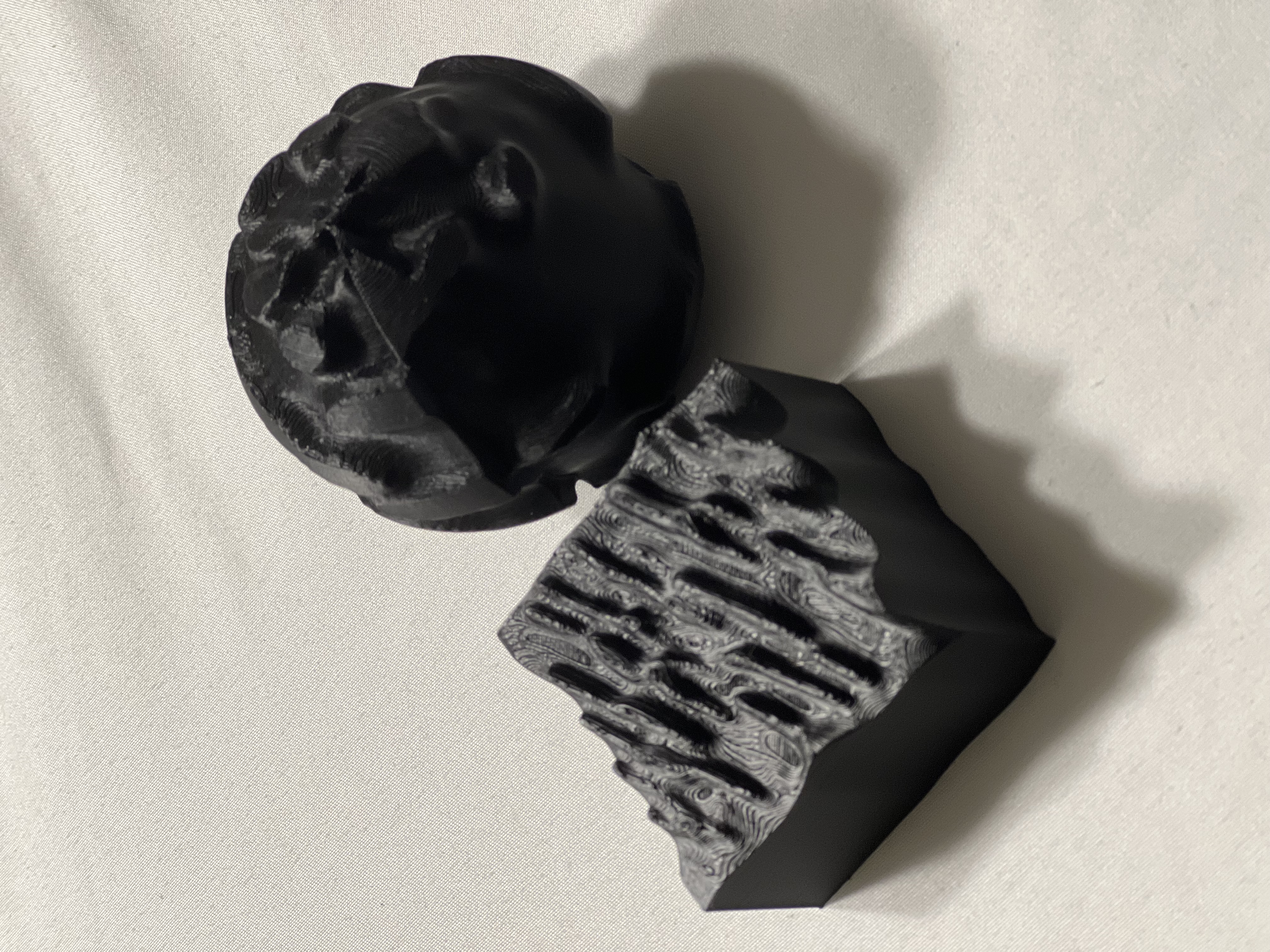
Here is the design I decided to print as an example. The full print can be seen in the next section.

Generating with Destroyer of Worlds by Ludwig Goransson.

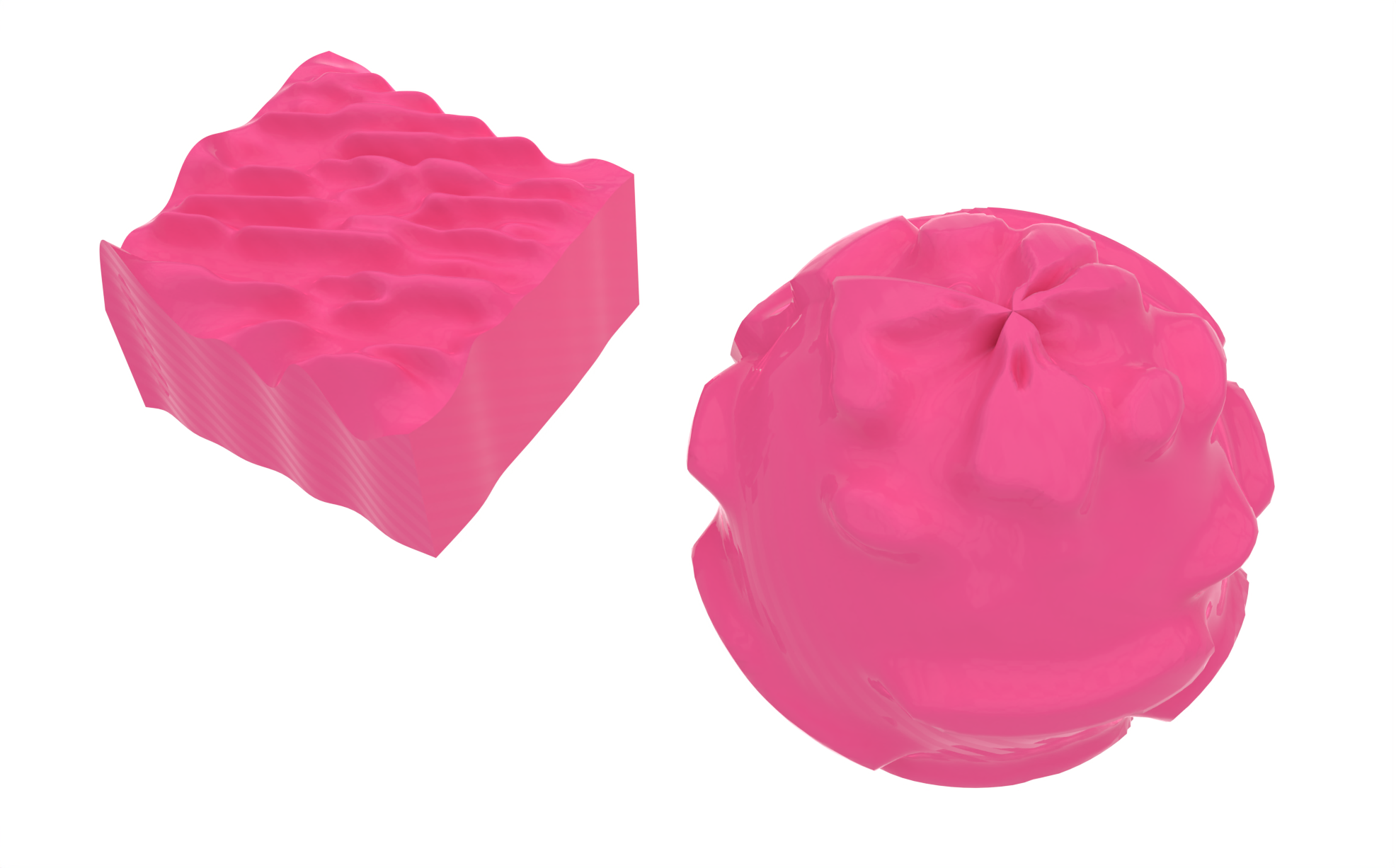
Print Result

Conclusions

At the beginning of this project, I had a lot of trouble since I was trying to find a way to incorporate marching cubes into the terrain generation algorithm. Eventually, I settled on forming a 2D matrix of displacement values using DFTs and directly adjusting vertices. This was simpler, and since audio is inherently time series data, a semi-continuous surface could be generated. Still, progress was rough since every miscalculation I made would cause Rhino and Grasshopper to crash due to the sheer amount of data in audio signals. I lost my progress nearly 20 times before I developed a habit of repeatedly saving after even minute changes.

I was quite satisfied with the outcome of this project, although I wish I had a little more time to refine the audio processing code. Currently, you can only select a specific window from the audio input to process. This is due to the limited number of vertices in the mesh. Too many crashes the program, so it’s normally not possible to display the entire audio on the surface of the objects, especially if the input is the length of a song. The method in place allows for the input window of the FFT to be changed using the sr_divider variable, which produces the window size by dividing the sample rate (normally 48 kHz). However, shrinking this value to get larger windows risks losing continuity since it spreads out the starting point of each FFT window. With further work, I would work on solving this issue by computing all FFTs across the input and interpolating values between them to match the number of vertices in the time dimension.

Another feature I would like to add is some text or other signifier of the original audio’s source onto the objects. At the moment, there’s no way to match up the appearance of the objects with their source audio without knowing what they are beforehand.